Player Recognition and Positioning Based on YOLOv5 and Resnet18

1. Research Objectives

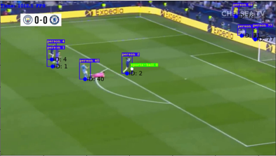
  To achieve the following functionality: Users submit a photo/video, specify the attacking team, defending team, referee, and the color of the ball. The model will automatically frame the ball and players, as well as the referee’s positions in the frame, and display their actual positions on a field coordinate map.

2. Research Methods

  Literature Review: In accordance with our research objectives, we gather ample information through the review of relevant literature to gain a comprehensive understanding of the background, history, current status, and prospects of the research topic.

  The following is our thought process through the literature review:

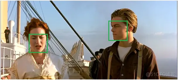
  Object detection is a critical problem in the field of computer vision. It involves detecting specific target objects in images and determining their positions and sizes. Such problems are highly valuable and can be applied to various practical applications such as face detection, vehicle detection, pedestrian detection, and more.

  Object detection problems can enhance the accuracy and precision of computer vision systems. For example, in autonomous driving systems, object detection can be used to detect other vehicles and pedestrians on the road for better vehicle control. In medical imaging, object detection can be employed to detect tumors, aiding doctors in disease diagnosis.

  The challenge in object detection lies in the fact that the positions, sizes, and shapes of target objects in images may vary, and images can be affected by occlusions, noise, and other disturbances. Therefore, solving object detection problems requires powerful models and algorithms capable of handling various scenarios. Currently, many deep learning models, such as Convolutional Neural Networks (CNNs), Residual Networks (ResNet), Single Anchor Box (YOLO), etc., can be used to tackle object detection problems.

  Hence, for this major project, our group chose to use the YOLOv5s model, a variant of the YOLOv5 model. Compared to the YOLOv5 model, YOLOv5s has smaller dimensions and faster speed but slightly lower accuracy. The YOLOv5s model is based on the Residual Network (ResNet) architecture and employs multiscale prediction for object detection and recognition. Its advantages lie in its small size and fast speed, making it suitable for use in mobile devices or embedded systems. However, due to its smaller model size, accuracy may be slightly reduced. Nevertheless, considering our available computational resources and the desired model scale, we have chosen to use the YOLOv5s model.

3. Algorithm Implementation

3.1 Problem Analysis

Core Problem:

  Given an image data (a soccer game), our model can perform object detection for players and the ball, while also tracking them. It generates anchor box results and projects them onto a 2D plane to create a projection matrix, providing the 2D positional information of players and the ball on the soccer field.

Problem Breakdown:

  1. We use YOLOv5s PyTorch for inference (loading a pre-trained YOLOv5s model).

  2. Implement tracking using the Deep SORT algorithm.

  3. Utilize a resnet-based model to generate a projection matrix for mapping to a 2D plane. (This model was trained on various soccer field footage and is part of an open-source project available at: https://github.com/vcg-uvic/sportsfield_release)

3.2 Data Collection

  Data is collected by scraping World Cup live TS files, converting them, and then labeling them.

  Typically, we would use a locally downloaded labeling tool for this task. However, considering that the labeled files need further conversion, our group opted to use readily available online tools. The following outlines the process of creating the dataset:

Access roboflow: https://roboflow.com/

Log in or register for an account.

Enter and create a new project after logging in:

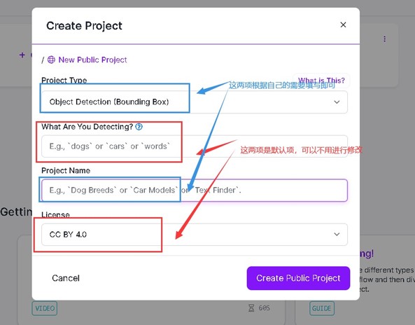
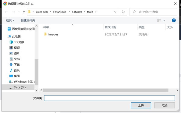
Select the folder where your local data is located:

Save your project here:

Allocate tasks:

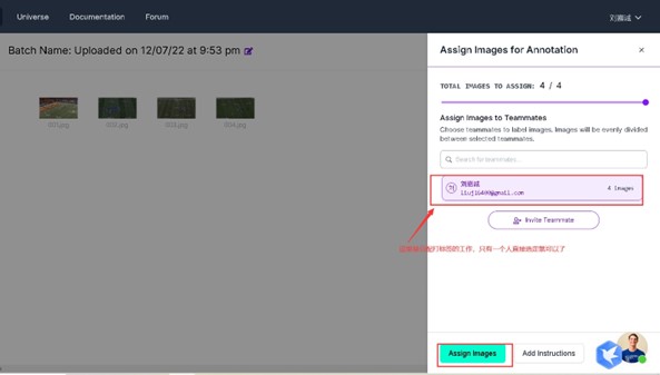
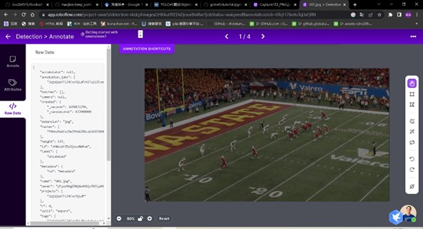
Access the work interface:

Click on an image to enter the labeling page:

Perform the labeling task:

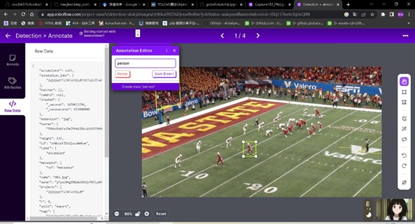
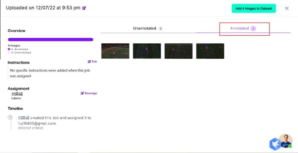
After labeling, it will be automatically saved, and you can see all the images with completed labels:

Allocate the dataset proportions:

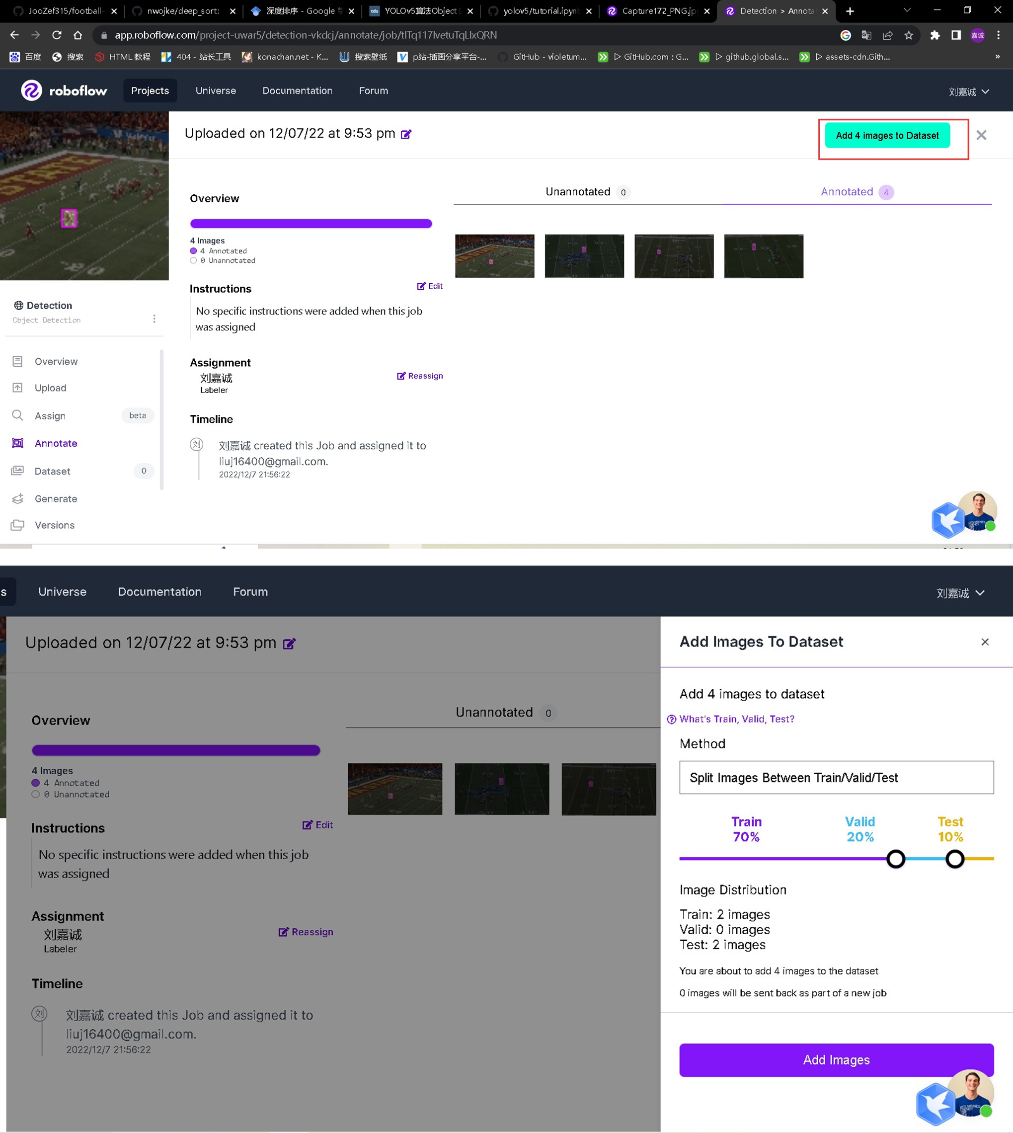
Reach the final step of the workflow:

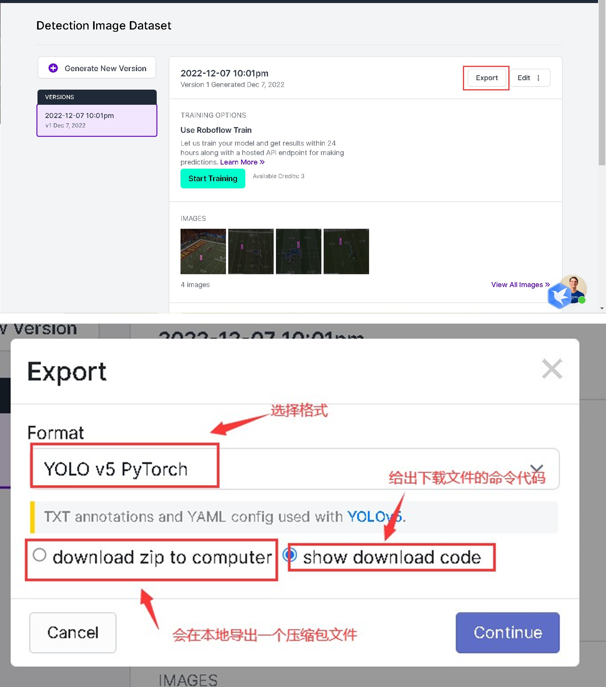
Click on “generate” on the left sidebar:

Generate the files:

Wait for the generation to complete:

Export the generated files:

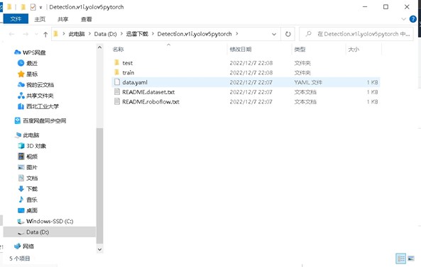
Directory of the generated files:

3.3 Model Establishment

3.3.1 Environment Setup

• Follow the instructions on the Huawei MindSpore official website to install MindSpore, and then use the MindSpore framework for model migration (environment setup).
• The model construction uses python3.7.5 and pytorch1.7.

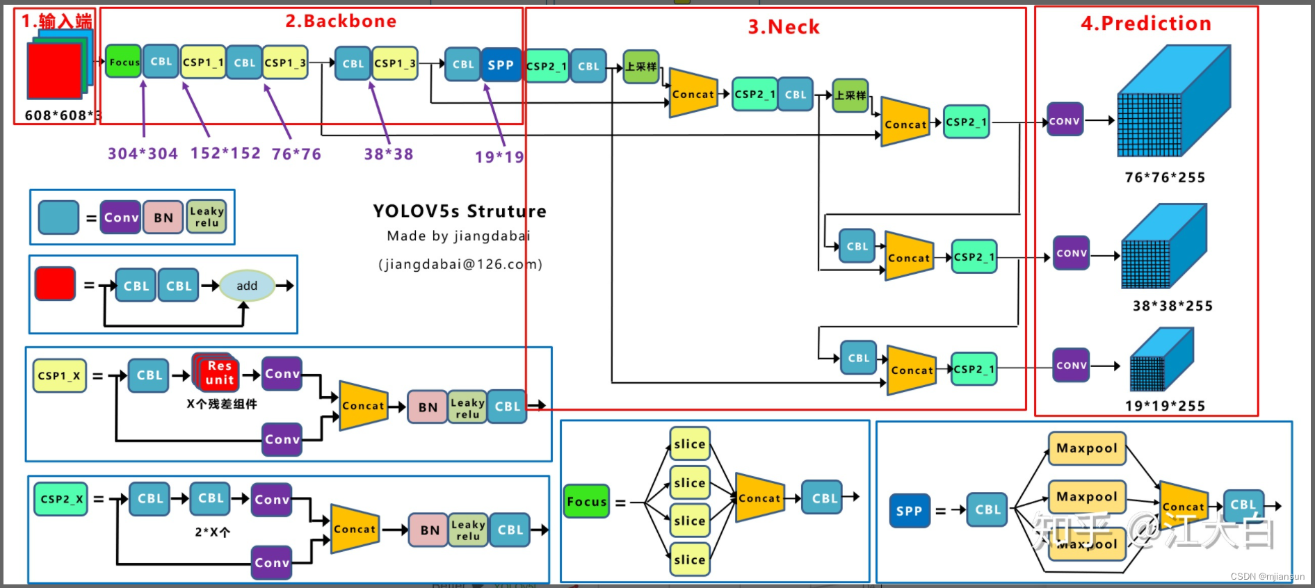
3.3.2 yolov5s Model Structure

3.3.2.1 Input End

• Mosaic Data Augmentation

  - First, let’s understand why we need to perform Mosaic data augmentation?

  In regular project training, the average precision (AP) of small targets is generally much lower than that of medium and large targets. The distribution of small targets is not uniform in the Coco dataset. First, let’s define small, medium, and large targets:

  In the 2019 paper titled “Augmentation for small object detection,” the distinction is made as follows:

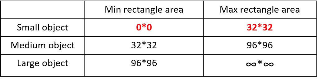
  In the Coco dataset, small targets account for 41.4%, with more in number compared to medium and large targets:

  In response to this situation, we choose to use Mosaic data augmentation.

• Mosaic data augmentation involves randomly using 4 images, randomly scaling them, and then randomly arranging them.

• Advantages:

  • Enriched dataset: Randomly using 4 images, random scaling, and then random arrangement significantly enrich the detection dataset, especially by adding many small targets, which improves the network’s robustness. Reduced GPU usage: Some may argue that random scaling can also be done with regular data augmentation. However, the authors considered that many people may have only one GPU. Therefore, during Mosaic augmentation training, the data for 4 images can be calculated directly, so the mini-batch size does not need to be very large, and good results can be achieved with just one GPU.

• Why does Mosaic data augmentation work well for small target detection?

  • Mosaic data augmentation can increase the diversity of images, enabling the model to better capture details in the images. This can improve the model’s ability to recognize small targets (corresponding to the advantage of an enriched dataset).
  • Mosaic data augmentation allows the model to learn the features of target objects at different scales. Since small target objects are relatively small in size, this method can better recognize small targets (corresponding to the operation of random scaling).
  • Mosaic data augmentation allows the model to generalize better. Since Mosaic data augmentation is achieved by randomly arranging small blocks, it can increase the model’s ability to handle new images. This can improve the detection performance of small targets by the model.

• # 源码实例, 拼四张图片
  def load_mosaic(self, index):
          # YOLOv5 4-mosaic loader. Loads 1 image + 3 random images into a 4-image mosaic
          labels4, segments4 = [], []
          s = self.img_size
          yc, xc = (int(random.uniform(-x, 2 * s + x)) for x in self.mosaic_border)  # mosaic center x, y
          indices = [index] + random.choices(self.indices, k=3)  # 3 additional image indices
          random.shuffle(indices)
          for i, index in enumerate(indices):
              # Load image
              img, _, (h, w) = self.load_image(index)
      
              # place img in img4
              if i == 0:  # top left
                  img4 = np.full((s * 2, s * 2, img.shape[2]), 114, dtype=np.uint8)  # base image with 4 tiles
                  x1a, y1a, x2a, y2a = max(xc - w, 0), max(yc - h, 0), xc, yc  # xmin, ymin, xmax, ymax (large image)
                  x1b, y1b, x2b, y2b = w - (x2a - x1a), h - (y2a - y1a), w, h  # xmin, ymin, xmax, ymax (small image)
              elif i == 1:  # top right
                  x1a, y1a, x2a, y2a = xc, max(yc - h, 0), min(xc + w, s * 2), yc
                  x1b, y1b, x2b, y2b = 0, h - (y2a - y1a), min(w, x2a - x1a), h
              elif i == 2:  # bottom left
                  x1a, y1a, x2a, y2a = max(xc - w, 0), yc, xc, min(s * 2, yc + h)
                  x1b, y1b, x2b, y2b = w - (x2a - x1a), 0, w, min(y2a - y1a, h)
              elif i == 3:  # bottom right
                  x1a, y1a, x2a, y2a = xc, yc, min(xc + w, s * 2), min(s * 2, yc + h)
                  x1b, y1b, x2b, y2b = 0, 0, min(w, x2a - x1a), min(y2a - y1a, h)
      
              img4[y1a:y2a, x1a:x2a] = img[y1b:y2b, x1b:x2b]  # img4[ymin:ymax, xmin:xmax]
              padw = x1a - x1b
              padh = y1a - y1b
      
              # Labels
              labels, segments = self.labels[index].copy(), self.segments[index].copy()
              if labels.size:
                  labels[:, 1:] = xywhn2xyxy(labels[:, 1:], w, h, padw, padh)  # normalized xywh to pixel xyxy format
                  segments = [xyn2xy(x, w, h, padw, padh) for x in segments]
              labels4.append(labels)
              segments4.extend(segments)
      
          # Concat/clip labels
          labels4 = np.concatenate(labels4, 0)
          for x in (labels4[:, 1:], *segments4):
              np.clip(x, 0, 2 * s, out=x)  # clip when using random_perspective()
          # img4, labels4 = replicate(img4, labels4)  # replicate
      
          # Augment
          img4, labels4, segments4 = copy_paste(img4, labels4, segments4, p=self.hyp['copy_paste'])
          img4, labels4 = random_perspective(img4,
                                             labels4,
                                             segments4,
                                             degrees=self.hyp['degrees'],
                                             translate=self.hyp['translate'],
                                             scale=self.hyp['scale'],
                                             shear=self.hyp['shear'],
                                             perspective=self.hyp['perspective'],
                                             border=self.mosaic_border)  # border to remove
      
          return img4, labels4
  

• # 源码实例, 拼九张图片
  def load_mosaic9(self, index):
          # YOLOv5 9-mosaic loader. Loads 1 image + 8 random images into a 9-image mosaic
          labels9, segments9 = [], []
          s = self.img_size
          indices = [index] + random.choices(self.indices, k=8)  # 8 additional image indices
          random.shuffle(indices)
          hp, wp = -1, -1  # height, width previous
          for i, index in enumerate(indices):
              # Load image
              img, _, (h, w) = self.load_image(index)
      
              # place img in img9
              if i == 0:  # center
                  img9 = np.full((s * 3, s * 3, img.shape[2]), 114, dtype=np.uint8)  # base image with 4 tiles
                  h0, w0 = h, w
                  c = s, s, s + w, s + h  # xmin, ymin, xmax, ymax (base) coordinates
              elif i == 1:  # top
                  c = s, s - h, s + w, s
              elif i == 2:  # top right
                  c = s + wp, s - h, s + wp + w, s
              elif i == 3:  # right
                  c = s + w0, s, s + w0 + w, s + h
              elif i == 4:  # bottom right
                  c = s + w0, s + hp, s + w0 + w, s + hp + h
              elif i == 5:  # bottom
                  c = s + w0 - w, s + h0, s + w0, s + h0 + h
              elif i == 6:  # bottom left
                  c = s + w0 - wp - w, s + h0, s + w0 - wp, s + h0 + h
              elif i == 7:  # left
                  c = s - w, s + h0 - h, s, s + h0
              elif i == 8:  # top left
                  c = s - w, s + h0 - hp - h, s, s + h0 - hp
      
              padx, pady = c[:2]
              x1, y1, x2, y2 = (max(x, 0) for x in c)  # allocate coords
      
              # Labels
              labels, segments = self.labels[index].copy(), self.segments[index].copy()
              if labels.size:
                  labels[:, 1:] = xywhn2xyxy(labels[:, 1:], w, h, padx, pady)  # normalized xywh to pixel xyxy format
                  segments = [xyn2xy(x, w, h, padx, pady) for x in segments]
              labels9.append(labels)
              segments9.extend(segments)
      
              # Image
              img9[y1:y2, x1:x2] = img[y1 - pady:, x1 - padx:]  # img9[ymin:ymax, xmin:xmax]
              hp, wp = h, w  # height, width previous
      
          # Offset
          yc, xc = (int(random.uniform(0, s)) for _ in self.mosaic_border)  # mosaic center x, y
          img9 = img9[yc:yc + 2 * s, xc:xc + 2 * s]
      
          # Concat/clip labels
          labels9 = np.concatenate(labels9, 0)
          labels9[:, [1, 3]] -= xc
          labels9[:, [2, 4]] -= yc
          c = np.array([xc, yc])  # centers
          segments9 = [x - c for x in segments9]
      
          for x in (labels9[:, 1:], *segments9):
              np.clip(x, 0, 2 * s, out=x)  # clip when using random_perspective()
          # img9, labels9 = replicate(img9, labels9)  # replicate
      
          # Augment
          img9, labels9, segments9 = copy_paste(img9, labels9, segments9, p=self.hyp['copy_paste'])
          img9, labels9 = random_perspective(img9,
                                             labels9,
                                             segments9,
                                             degrees=self.hyp['degrees'],
                                             translate=self.hyp['translate'],
                                             scale=self.hyp['scale'],
                                             shear=self.hyp['shear'],
                                             perspective=self.hyp['perspective'],
                                             border=self.mosaic_border)  # border to remove
      
          return img9, labels9
  

• Adaptive Anchor Box Calculation

  • For different datasets, anchor boxes are computed as priors. During network training, the network makes predictions based on these anchors, then outputs predicted boxes, and finally compares them with the labeled boxes, followed by gradient-based backpropagation.

  • In YOLOv3 and YOLOv4, when training on different datasets, a separate script is used to initially calculate anchor boxes. However, in YOLOv5, this functionality is embedded within the entire training code. Therefore, before each training session, YOLOv5 adaptively calculates anchors based on the specific dataset.

  • The specific process of adaptive anchor calculation is as follows:

    1. Get the width and height of all the targets in the dataset.
    2. Resize each image proportionally to the specified size, ensuring that the maximum value among width and height matches the specified size.
    3. Convert bounding boxes (bboxes) from relative coordinates to absolute coordinates, scaling them by the resized width and height.
    4. Filter bboxes, retaining those with width and height both greater than or equal to two pixels.
    5. Use k-means clustering to obtain n anchors, following the same procedure as in v3 and v4.
    6. Randomly mutate the width and height of anchors using a genetic algorithm. If the mutated result improves, it is assigned to the anchors; if the result worsens, it is skipped. By default, mutation is attempted 1000 times. The anchor fitness is calculated using the anchor_fitness method and then evaluated.

    import random
        
    import numpy as np
    import torch
    import yaml
    from tqdm import tqdm
        
    from utils import TryExcept
    from utils.general import LOGGER, TQDM_BAR_FORMAT, colorstr
        
    PREFIX = colorstr('AutoAnchor: ')
        
        
    def check_anchor_order(m):
        # Check anchor order against stride order for YOLOv5 Detect() module m, and correct if necessary
        a = m.anchors.prod(-1).mean(-1).view(-1)  # mean anchor area per output layer
        da = a[-1] - a[0]  # delta a
        ds = m.stride[-1] - m.stride[0]  # delta s
        if da and (da.sign() != ds.sign()):  # same order
            LOGGER.info(f'{PREFIX}Reversing anchor order')
            m.anchors[:] = m.anchors.flip(0)
        
        
    @TryExcept(f'{PREFIX}ERROR')
    def check_anchors(dataset, model, thr=4.0, imgsz=640):
        # Check anchor fit to data, recompute if necessary
        m = model.module.model[-1] if hasattr(model, 'module') else model.model[-1]  # Detect()
        shapes = imgsz * dataset.shapes / dataset.shapes.max(1, keepdims=True)
        scale = np.random.uniform(0.9, 1.1, size=(shapes.shape[0], 1))  # augment scale
        wh = torch.tensor(np.concatenate([l[:, 3:5] * s for s, l in zip(shapes * scale, dataset.labels)])).float()  # wh
        
        def metric(k):  # compute metric
            r = wh[:, None] / k[None]
            x = torch.min(r, 1 / r).min(2)[0]  # ratio metric
            best = x.max(1)[0]  # best_x
            aat = (x > 1 / thr).float().sum(1).mean()  # anchors above threshold
            bpr = (best > 1 / thr).float().mean()  # best possible recall
            return bpr, aat
        
        stride = m.stride.to(m.anchors.device).view(-1, 1, 1)  # model strides
        anchors = m.anchors.clone() * stride  # current anchors
        bpr, aat = metric(anchors.cpu().view(-1, 2))
        s = f'\n{PREFIX}{aat:.2f} anchors/target, {bpr:.3f} Best Possible Recall (BPR). '
        if bpr > 0.98:  # threshold to recompute
            LOGGER.info(f'{s}Current anchors are a good fit to dataset ✅')
        else:
            LOGGER.info(f'{s}Anchors are a poor fit to dataset ⚠️, attempting to improve...')
            na = m.anchors.numel() // 2  # number of anchors
            anchors = kmean_anchors(dataset, n=na, img_size=imgsz, thr=thr, gen=1000, verbose=False)
            new_bpr = metric(anchors)[0]
            if new_bpr > bpr:  # replace anchors
                anchors = torch.tensor(anchors, device=m.anchors.device).type_as(m.anchors)
                m.anchors[:] = anchors.clone().view_as(m.anchors)
                check_anchor_order(m)  # must be in pixel-space (not grid-space)
                m.anchors /= stride
                s = f'{PREFIX}Done ✅ (optional: update model *.yaml to use these anchors in the future)'
            else:
                s = f'{PREFIX}Done ⚠️ (original anchors better than new anchors, proceeding with original anchors)'
            LOGGER.info(s)
        
        
    def kmean_anchors(dataset='./data/coco128.yaml', n=9, img_size=640, thr=4.0, gen=1000, verbose=True):
        """ Creates kmeans-evolved anchors from training dataset
        
            Arguments:
                dataset: path to data.yaml, or a loaded dataset
                n: number of anchors
                img_size: image size used for training
                thr: anchor-label wh ratio threshold hyperparameter hyp['anchor_t'] used for training, default=4.0
                gen: generations to evolve anchors using genetic algorithm
                verbose: print all results
        
            Return:
                k: kmeans evolved anchors
        
            Usage:
                from utils.autoanchor import *; _ = kmean_anchors()
        """
        from scipy.cluster.vq import kmeans
        
        npr = np.random
        thr = 1 / thr
        
        def metric(k, wh):  # compute metrics
            r = wh[:, None] / k[None]
            x = torch.min(r, 1 / r).min(2)[0]  # ratio metric
            # x = wh_iou(wh, torch.tensor(k))  # iou metric
            return x, x.max(1)[0]  # x, best_x
        
        def anchor_fitness(k):  # mutation fitness
            _, best = metric(torch.tensor(k, dtype=torch.float32), wh)
            return (best * (best > thr).float()).mean()  # fitness
        
        def print_results(k, verbose=True):
            k = k[np.argsort(k.prod(1))]  # sort small to large
            x, best = metric(k, wh0)
            bpr, aat = (best > thr).float().mean(), (x > thr).float().mean() * n  # best possible recall, anch > thr
            s = f'{PREFIX}thr={thr:.2f}: {bpr:.4f} best possible recall, {aat:.2f} anchors past thr\n' \
                f'{PREFIX}n={n}, img_size={img_size}, metric_all={x.mean():.3f}/{best.mean():.3f}-mean/best, ' \
                f'past_thr={x[x > thr].mean():.3f}-mean: '
            for x in k:
                s += '%i,%i, ' % (round(x[0]), round(x[1]))
            if verbose:
                LOGGER.info(s[:-2])
            return k
        
        if isinstance(dataset, str):  # *.yaml file
            with open(dataset, errors='ignore') as f:
                data_dict = yaml.safe_load(f)  # model dict
            from utils.dataloaders import LoadImagesAndLabels
            dataset = LoadImagesAndLabels(data_dict['train'], augment=True, rect=True)
        
        # Get label wh
        shapes = img_size * dataset.shapes / dataset.shapes.max(1, keepdims=True)
        wh0 = np.concatenate([l[:, 3:5] * s for s, l in zip(shapes, dataset.labels)])  # wh
        
        # Filter
        i = (wh0 < 3.0).any(1).sum()
        if i:
            LOGGER.info(f'{PREFIX}WARNING ⚠️ Extremely small objects found: {i} of {len(wh0)} labels are <3 pixels in size')
        wh = wh0[(wh0 >= 2.0).any(1)].astype(np.float32)  # filter > 2 pixels
        # wh = wh * (npr.rand(wh.shape[0], 1) * 0.9 + 0.1)  # multiply by random scale 0-1
        
        # Kmeans init
        try:
            LOGGER.info(f'{PREFIX}Running kmeans for {n} anchors on {len(wh)} points...')
            assert n <= len(wh)  # apply overdetermined constraint
            s = wh.std(0)  # sigmas for whitening
            k = kmeans(wh / s, n, iter=30)[0] * s  # points
            assert n == len(k)  # kmeans may return fewer points than requested if wh is insufficient or too similar
        except Exception:
            LOGGER.warning(f'{PREFIX}WARNING ⚠️ switching strategies from kmeans to random init')
            k = np.sort(npr.rand(n * 2)).reshape(n, 2) * img_size  # random init
        wh, wh0 = (torch.tensor(x, dtype=torch.float32) for x in (wh, wh0))
        k = print_results(k, verbose=False)
        
        # Plot
        # k, d = [None] * 20, [None] * 20
        # for i in tqdm(range(1, 21)):
        #     k[i-1], d[i-1] = kmeans(wh / s, i)  # points, mean distance
        # fig, ax = plt.subplots(1, 2, figsize=(14, 7), tight_layout=True)
        # ax = ax.ravel()
        # ax[0].plot(np.arange(1, 21), np.array(d) ** 2, marker='.')
        # fig, ax = plt.subplots(1, 2, figsize=(14, 7))  # plot wh
        # ax[0].hist(wh[wh[:, 0]<100, 0],400)
        # ax[1].hist(wh[wh[:, 1]<100, 1],400)
        # fig.savefig('wh.png', dpi=200)
        
        # Evolve
        f, sh, mp, s = anchor_fitness(k), k.shape, 0.9, 0.1  # fitness, generations, mutation prob, sigma
        pbar = tqdm(range(gen), bar_format=TQDM_BAR_FORMAT)  # progress bar
        for _ in pbar:
            v = np.ones(sh)
            while (v == 1).all():  # mutate until a change occurs (prevent duplicates)
                v = ((npr.random(sh) < mp) * random.random() * npr.randn(*sh) * s + 1).clip(0.3, 3.0)
            kg = (k.copy() * v).clip(min=2.0)
            fg = anchor_fitness(kg)
            if fg > f:
                f, k = fg, kg.copy()
                pbar.desc = f'{PREFIX}Evolving anchors with Genetic Algorithm: fitness = {f:.4f}'
                if verbose:
                    print_results(k, verbose)
        
        return print_results(k).astype(np.float32)
    

• Adaptive Image Resizing

  • In commonly used object detection algorithms, images often have different dimensions. Therefore, a common practice is to resize all original images to a standard size before feeding them into the detection network. In practical applications, many images have varying aspect ratios, resulting in different amounts of black borders at the top and bottom after resizing and padding. Excessive padding can lead to redundant information and impact inference speed. Adaptive image resizing is employed to improve inference speed.

  • The calculation steps are as follows:

    • Step 1: Calculate the scaling ratio The original resizing size is 416x416. After dividing the original image dimensions by these values, two scaling factors, 0.52 and 0.69, are obtained. The smaller scaling factor is chosen.

    • Step 2: Calculate the resized dimensions Multiplying the original image dimensions by the smallest scaling factor, 0.52, results in a width of 416 and a height of 312.

    • Step 3: Calculate the padding values for black borders The original image’s height needs to be padded by 416 - 312 = 104 pixels. Using the np.mod function in numpy to calculate the remainder results in 8 pixels, which, when divided by 2, gives the number of pixels to be padded on each side of the image’s height.

3.3.2.2、Backbone

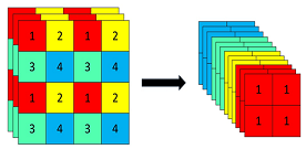
• Focus Structure:

  # 代码实例
  class Focus(nn.Module):
      # Focus wh information into c-space
      def __init__(self, c1, c2, k=1, s=1, p=None, g=1, act=True):  # ch_in, ch_out, kernel, stride, padding, groups
          super().__init__()
          self.conv = Conv(c1 * 4, c2, k, s, p, g, act=act)
          # self.contract = Contract(gain=2)
    
      def forward(self, x):  # x(b,c,w,h) -> y(b,4c,w/2,h/2)
          return self.conv(torch.cat((x[..., ::2, ::2], x[..., 1::2, ::2], x[..., ::2, 1::2], x[..., 1::2, 1::2]), 1))
          # return self.conv(self.contract(x))
  

  

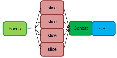
The original image of size 640 × 640 × 3 is input into the Focus structure, which undergoes a slicing operation, first transforming into a feature map of size 320 × 320 × 12, and then going through a convolution operation to finally become a feature map of size 320 × 320 × 32. The slicing operation is illustrated as follows:

Purpose: The main purpose of the Focus layer is to reduce the number of layers, parameters, FLOPS (computational load), CUDA memory usage, and improve forward and backward speeds, all while minimizing its impact on mAP (mean Average Precision). (Source: Author’s documentation)

• Reducing Layers, Parameters, and FLOPS (Computational Load):

  To provide a comparison:

  Regular downsampling: Inputting a 640 × 640 × 3 image into a 3 × 3 convolution with a stride of 2 and an output channel of 32, results in a downsampled feature map of size 320 × 320 × 32. The theoretical computational load for this regular convolution downsample is:

  FLOPs (conv) = 3 × 3 × 3 × 32 × 320 × 320 = 88,473,600 (without considering bias) Parameters (conv) = 3 × 3 × 3 × 32 + 32 + 32 = 928 (where the last two 32s represent bias and BN layer parameters, respectively)

  Focus: Inputting a 640 × 640 × 3 image into the Focus structure, which employs a slicing operation to transform it into a feature map of size 320 × 320 × 12, followed by a 3 × 3 convolution operation with an output channel of 32, resulting in a feature map of size 320 × 320 × 32. The theoretical computational load for the Focus layer is:

  FLOPs (Focus) = 3 × 3 × 12 × 32 × 320 × 320 = 353,894,400 (without considering bias) Parameters (Focus) = 3 × 3 × 12 × 32 + 32 + 32 = 3,520 (To account for bias and BN layer parameters, although these typically have a relatively small impact and can be ignored.)

• Reducing CUDA Memory Usage, Improving Forward and Backward Speeds, and Minimizing Impact on mAP:

  After extensive analysis of alternative designs for the YOLOv3 input layer, the author decided to adopt the current Focus layer design. This decision was made to obtain immediate forward/backward/memory analysis results and to compare it with a complete 300-epoch COCO training to determine its impact on mAP. The Focus layer was analyzed based on the original YOLOv3 layer, and this decision was made to optimize YOLOv5’s performance.

  ```python
  # Profile
  import torch.nn as nn
  from models.common import Focus, Conv, Bottleneck
  from utils.torch_utils import profile 
    
  m1 = Focus(3, 64, 3)  # YOLOv5 Focus layer
  m2 = nn.Sequential(Conv(3, 32, 3, 1), Conv(32, 64, 3, 2), Bottleneck(64, 64))  # YOLOv3 first 3 layers
    
  results = profile(input=torch.randn(16, 3, 640, 640), ops=[m1, m2], n=10, device=0)  # profile both 10 times at batch-size 16
  ```
      
  得到结果：
      
  显卡`device=0`
      
  ```
  YOLOv5 🚀 v5.0-405-gfad57c2 torch 1.9.0+cu102 CUDA:0 (Tesla T4, 15109.75MB)
    
  Params   GFLOPs  GPU_mem (GB)  forward (ms) backward (ms)  
  7040     23.07   2.259     	   16.65        54.1                  
  input               output
  (16, 3, 640, 640)  (16, 64, 320, 320)  
  # Focus
  Params   GFLOPs  GPU_mem (GB)  forward (ms) backward (ms)
  40160    140.7   7.522         77.86        331.9
  input               output       	      
  (16, 3, 640, 640)  (16, 64, 320, 320)
  ```
      
  中央处理器`device='cpu'`
      
  ```
  Params      GFLOPs  GPU_mem (GB)  forward (ms) backward (ms)
  7040        23.07   0.000         882.1        2029       	 
  input        		output
  (16, 3, 640, 640)      (16, 64, 320, 320) 
  # Focus
  Params      GFLOPs  GPU_mem (GB)  forward (ms) backward (ms)
  40160       140.7   0.000         4513         8565       
  input        		output
  (16, 3, 640, 640)   (16, 64, 320, 320)
  ```
  

• CSP Structure:

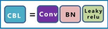
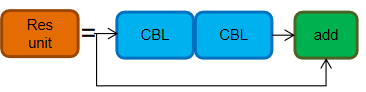
  • CBL (Convolution, Batch Normalization, Leaky ReLU): A CBL unit is composed of Convolution, Batch Normalization, and Leaky ReLU activation.

    

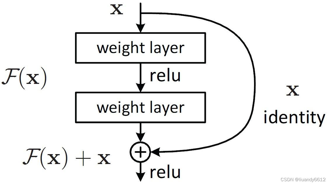
  • Res Unit: The Res unit is designed based on the concept of residual structures.

    

    

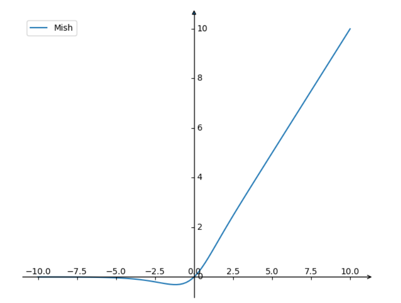
  • CBM (Convolution, Batch Normalization, Mish Activation): CBM is a sub-module within the residual module, consisting of Convolution, Batch Normalization, and the Mish activation function.

    \[f(x)=x \cdot \tanh \left(\ln \left(1+e^x\right)\right)\]

    

    The plot above illustrates the Mish activation function. It shares similarities with ReLU by having no upper bound, which helps prevent gradient saturation. Additionally, the Mish function is smooth everywhere and allows some negative values in the region of small absolute values.

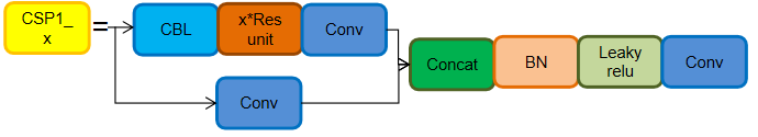
  • CSP1_X: Derived from CSPNet, this module consists of CBL modules, Res units, Convolutions, and Concatenation. The ‘X’ denotes that there are ‘X’ instances of this module.

    

    • Adding residual structures enhances the gradient flow between layers, preventing gradient vanishing and allowing for feature extraction at finer scales without concerns of network degradation.

  • Role of CSP1_X:

    • Improved Feature Extraction: By combining the main and auxiliary branches, CSP1_X captures complex structures and details in the image, transforming them into low-dimensional feature representations. This enhances the model’s recognition capabilities for target objects.

    • Enhanced Multi-scale Capability: Through the branch’s convolution layers, CSP1_X captures features of the target object at different scales, converting them into multiple feature maps. Ultimately, these feature maps are concatenated together and used in convolution layers, activation functions, and detection layers to predict the position and size of target objects.

    • Efficiency: CSP1_X has fewer branches, resulting in fewer parameters and faster training speeds. However, due to the reduced number of convolution layers in the branches, its feature extraction capabilities are relatively lower. Therefore, while CSP1_X models maintain speed advantages, there may be a slight decrease in accuracy (a trade-off).

    • 3.3.2.3、neck

• SPP Module (SPPF Module)

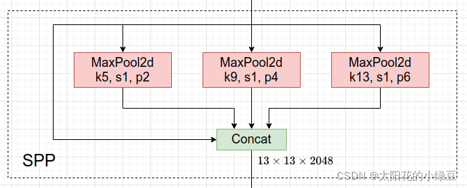
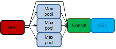
  • SPP (Spatial Pyramid Pooling): SPP has been used in YOLOv3 and later versions. SPP is a module that performs multiscale feature fusion by employing max-pooling operations of different sizes, specifically 1 × 1, 5 × 5, 9 × 9, and 13 × 13.

  • 

    

    class SPP(nn.Module):
        # Spatial Pyramid Pooling (SPP) layer https://arxiv.org/abs/1406.4729
        def __init__(self, c1, c2, k=(5, 9, 13)):
            super().__init__()
            c_ = c1 // 2  # hidden channels
            self.cv1 = Conv(c1, c_, 1, 1)
            self.cv2 = Conv(c_ * (len(k) + 1), c2, 1, 1)
            self.m = nn.ModuleList([nn.MaxPool2d(kernel_size=x, stride=1, padding=x // 2) for x in k])
        
        def forward(self, x):
            x = self.cv1(x)
            with warnings.catch_warnings():
                warnings.simplefilter('ignore')  # suppress torch 1.9.0 max_pool2d() warning
                return self.cv2(torch.cat([x] + [m(x) for m in self.m], 1))
    

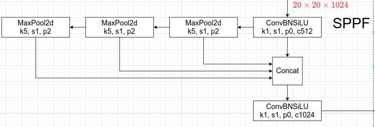
• In the new version of YOLOv5, an upgraded version of the SPP structure, known as SPPF, is used. SPPF replaces the parallel MaxPool operations with sequential MaxPool operations. Specifically, two sequential 5 × 5 MaxPool layers and one 9 × 9 MaxPool layer are equivalent to the parallel configuration, and three sequential 5 × 5 MaxPool layers are equivalent to one 13 × 13 MaxPool layer. Both parallel and sequential configurations achieve the same effect, but the sequential configuration is more efficient.
  • 

    class SPPF(nn.Module):
        # Spatial Pyramid Pooling - Fast (SPPF) layer for YOLOv5 by Glenn Jocher
        def __init__(self, c1, c2, k=5):  # equivalent to SPP(k=(5, 9, 13))
            super().__init__()
            c_ = c1 // 2  # hidden channels
            self.cv1 = Conv(c1, c_, 1, 1)
            self.cv2 = Conv(c_ * 4, c2, 1, 1)
            self.m = nn.MaxPool2d(kernel_size=k, stride=1, padding=k // 2)
      
        def forward(self, x):
            x = self.cv1(x)
            with warnings.catch_warnings():
                warnings.simplefilter('ignore')  # suppress torch 1.9.0 max_pool2d() warning
                y1 = self.m(x)
                y2 = self.m(y1)
                return self.cv2(torch.cat((x, y1, y2, self.m(y2)), 1))
  

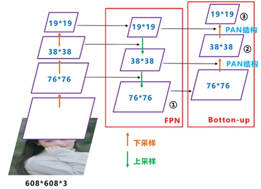
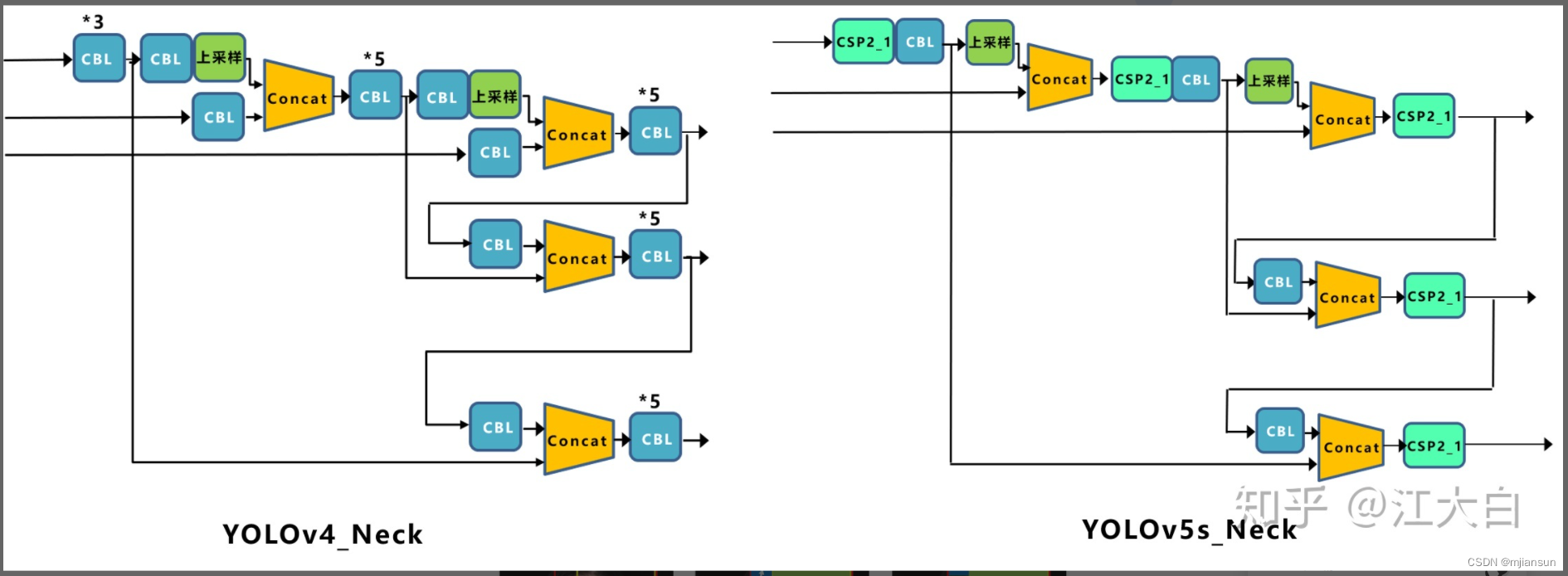
• YOLOv5 now uses the same Neck architecture as YOLOv4, which is based on the FPN (Feature Pyramid Network) and PAN (Path Aggregation Network) structures.

  • FPN (Feature Pyramid Network):

    First, let’s examine various convolutional classification methods:

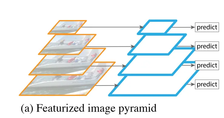
    • Image pyramids, which involve computing and memory overhead.

    

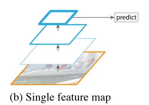
    • Simple classification networks like AlexNet that may not capture small objects.

    

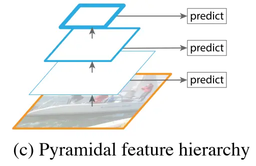
    • Pyramidal feature hierarchy, which has less semantic information in the lower-scale feature maps but may capture smaller objects.

    

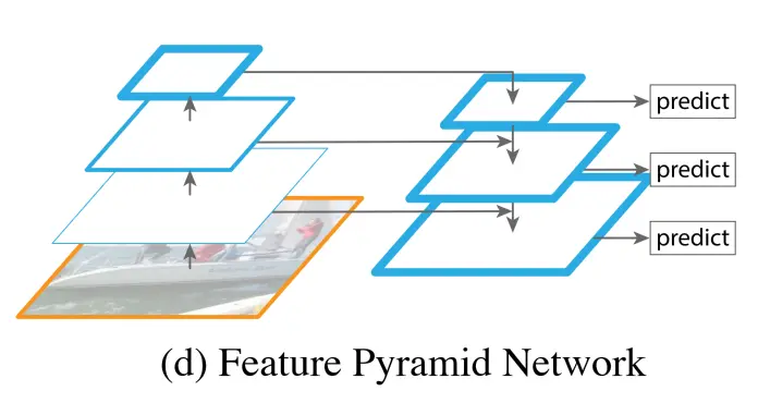
    • The Feature Pyramid Network (FPN) aims to address the issue of varying semantic information and spatial resolution in feature maps. FPN first conducts traditional bottom-up feature extraction, and then it tries to merge adjacent feature maps on the left side. The left side is referred to as “bottom-up,” the right side as “top-down,” and the horizontal connections are known as “lateral connections.” This approach is used because high-level feature maps have more semantics, while low-level feature maps have less semantics but more positional information.

    

    • Problem solved by FPN: While this works well for detecting large objects, it has limitations in detecting small objects. For small objects, as we perform convolution and pooling to reach the final layer, the semantic information is lost because the mapping to a feature map is achieved by directly dividing the coordinates by the stride. As we move to higher layers, the mapping may become too small or even non-existent. To address the issue of multi-scale detection, the Feature Pyramid Network (FPN) was introduced.

    • '''FPN in PyTorch.
              
      See the paper "Feature Pyramid Networks for Object Detection" for more details.
      '''
      import torch
      import torch.nn as nn
      import torch.nn.functional as F
              
      from torch.autograd import Variable
              
              
      class Bottleneck(nn.Module):
          expansion = 4
              
          def __init__(self, in_planes, planes, stride=1):
              super(Bottleneck, self).__init__()
              self.conv1 = nn.Conv2d(in_planes, planes, kernel_size=1, bias=False)
              self.bn1 = nn.BatchNorm2d(planes)
              self.conv2 = nn.Conv2d(planes, planes, kernel_size=3, stride=stride, padding=1, bias=False)
              self.bn2 = nn.BatchNorm2d(planes)
              self.conv3 = nn.Conv2d(planes, self.expansion*planes, kernel_size=1, bias=False)
              self.bn3 = nn.BatchNorm2d(self.expansion*planes)
              
              self.shortcut = nn.Sequential()
              if stride != 1 or in_planes != self.expansion*planes:
                  self.shortcut = nn.Sequential(
                      nn.Conv2d(in_planes, self.expansion*planes, kernel_size=1, stride=stride, bias=False),
                      nn.BatchNorm2d(self.expansion*planes)
                  )
              
          def forward(self, x):
              out = F.relu(self.bn1(self.conv1(x)))
              out = F.relu(self.bn2(self.conv2(out)))
              out = self.bn3(self.conv3(out))
              out += self.shortcut(x)
              out = F.relu(out)
              return out
              
              
      class FPN(nn.Module):
          def __init__(self, block, num_blocks):
              super(FPN, self).__init__()
              self.in_planes = 64
              
              self.conv1 = nn.Conv2d(3, 64, kernel_size=7, stride=2, padding=3, bias=False)
              self.bn1 = nn.BatchNorm2d(64)
              
              # Bottom-up layers
              self.layer1 = self._make_layer(block,  64, num_blocks[0], stride=1)
              self.layer2 = self._make_layer(block, 128, num_blocks[1], stride=2)
              self.layer3 = self._make_layer(block, 256, num_blocks[2], stride=2)
              self.layer4 = self._make_layer(block, 512, num_blocks[3], stride=2)
              
              # Top layer
              self.toplayer = nn.Conv2d(2048, 256, kernel_size=1, stride=1, padding=0)  # Reduce channels
              
              # Smooth layers
              self.smooth1 = nn.Conv2d(256, 256, kernel_size=3, stride=1, padding=1)
              self.smooth2 = nn.Conv2d(256, 256, kernel_size=3, stride=1, padding=1)
              self.smooth3 = nn.Conv2d(256, 256, kernel_size=3, stride=1, padding=1)
              
              # Lateral layers
              self.latlayer1 = nn.Conv2d(1024, 256, kernel_size=1, stride=1, padding=0)
              self.latlayer2 = nn.Conv2d( 512, 256, kernel_size=1, stride=1, padding=0)
              self.latlayer3 = nn.Conv2d( 256, 256, kernel_size=1, stride=1, padding=0)
              
          def _make_layer(self, block, planes, num_blocks, stride):
              strides = [stride] + [1]*(num_blocks-1)
              layers = []
              for stride in strides:
                  layers.append(block(self.in_planes, planes, stride))
                  self.in_planes = planes * block.expansion
              return nn.Sequential(*layers)
              
          def _upsample_add(self, x, y):
              '''Upsample and add two feature maps.
              
              Args:
                x: (Variable) top feature map to be upsampled.
                y: (Variable) lateral feature map.
              
              Returns:
                (Variable) added feature map.
              
              Note in PyTorch, when input size is odd, the upsampled feature map
              with `F.upsample(..., scale_factor=2, mode='nearest')`
              maybe not equal to the lateral feature map size.
              
              e.g.
              original input size: [N,_,15,15] ->
              conv2d feature map size: [N,_,8,8] ->
              upsampled feature map size: [N,_,16,16]
              
              So we choose bilinear upsample which supports arbitrary output sizes.
              '''
              _,_,H,W = y.size()
              return F.upsample(x, size=(H,W), mode='bilinear') + y
              
          def forward(self, x):
              # Bottom-up
              c1 = F.relu(self.bn1(self.conv1(x)))
              c1 = F.max_pool2d(c1, kernel_size=3, stride=2, padding=1)
              c2 = self.layer1(c1)
              c3 = self.layer2(c2)
              c4 = self.layer3(c3)
              c5 = self.layer4(c4)
              # Top-down
              p5 = self.toplayer(c5)
              p4 = self._upsample_add(p5, self.latlayer1(c4))
              p3 = self._upsample_add(p4, self.latlayer2(c3))
              p2 = self._upsample_add(p3, self.latlayer3(c2))
              # Smooth
              p4 = self.smooth1(p4)
              p3 = self.smooth2(p3)
              p2 = self.smooth3(p2)
              return p2, p3, p4, p5
      

  • PAN

• FPN (Feature Pyramid Network) is a top-down feature pyramid that enhances the entire pyramid by passing down strong semantic features from higher layers. However, it only enhances semantic information without conveying localization information effectively (or the transmission of localization information is not very effective due to the long path). PAN (Path Aggregation Network) addresses this limitation by adding a bottom-up pyramid to FPN, complementing FPN by passing low-level localization features upwards. This combined pyramid incorporates both semantic and localization information.

  

• To create PAN on top of the feature pyramid formed by FPN (top-down feature pyramid), the following operations are performed:

  (1) First, the bottom-most layer of the feature pyramid is duplicated (①) to become the bottom layer of the new feature pyramid.

  (2) The bottom layer of the new feature pyramid undergoes a downsampling operation. Then, the second-to-last layer of the original feature pyramid undergoes a 3 x 3 convolution with a stride of 2. The result is then combined with the downsampled bottom layer using lateral connections, followed by a 3 x 3 convolution to fuse their features.

  (3) The operations for the other layers of the new feature pyramid are the same as in (2).

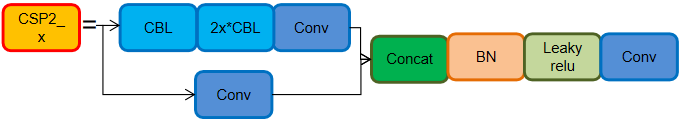
• The difference between YOLOv5 and YOLOv4 lies in CSP2_X, which enhances the network’s feature fusion capability:

  

  • CSP2_X is also composed of a CSPNet network, consisting of Conv layers and X Res units concatenated.

  

3.3.2.4 Output

• Bounding Box Loss Function:

  • YOLOv5 uses the CIOU_Loss as the bounding box loss function.

\[\text{CIOU_Loss} = 1 - \text{CIOU} = 1 - \left(\text{IOU} - \frac{\text{Distance}^2}{\text{Distance_}^2} - \frac{v^2}{(1 - \text{IOU}) + v}\right)\]

Where v is defined as:

\[v = \frac{4}{\pi^2}\left(\arctan \frac{\mathrm{w}^{\mathrm{gt}}}{\mathrm{h}^{\mathrm{gt}}} - \arctan \frac{\mathrm{w}^{\mathrm{p}}}{\mathrm{h}^{\mathrm{p}}}\right)^2\]

In this way, CIOU_Loss takes into account three important geometric factors for bounding box regression: overlap area, center point distance, and aspect ratio.

Comparing the differences between various loss functions:

• IOU_Loss: Primarily focuses on the overlap area between the detection box and the target box.
• GIOU_Loss: Builds upon IOU by addressing the issue of non-overlapping bounding boxes.
• DIOU_Loss: Extends IOU and GIOU by considering the distance between the center points of bounding boxes.

• CIOU_Loss: Expands upon DIOU by incorporating information about the aspect ratio of bounding boxes.

• NMS (Non-Maximum Suppression):

  NMS is a technique commonly used in recent object detection algorithms (including RCNN, SPPNet, Fast R-CNN, Faster R-CNN, etc.) to filter out redundant bounding boxes and select the most relevant ones. Here’s how NMS works:

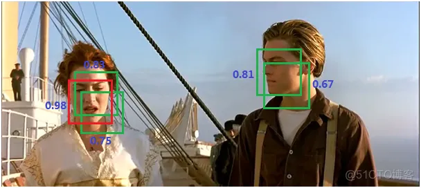
  (1) All bounding boxes are sorted based on their scores, and the one with the highest score is selected.

  (2) The remaining boxes are iterated through, and if the overlap area (IOU) with the currently selected highest-score box exceeds a certain threshold, those boxes are removed. This is done to keep only one box per object (assuming they belong to the same category).

  (3) The process continues by selecting the highest-scoring box from the remaining unprocessed boxes.

  Here’s an example:

  (1) Sorting all boxes by score and selecting the highest-scoring one:

  

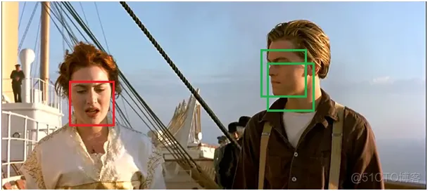
  (2) Iterating through the remaining boxes and removing those with IOU above the threshold:

  

  (3) Continuing to select the highest-scoring box from the remaining ones:

  

3.4 Attention Mechanism (SE) Integration into the Model

The Attention Mechanism (Attention Mechanism) is derived from the study of human vision. The attention mechanism mainly involves two aspects: determining which part of the input needs attention and allocating limited information processing resources to important parts.

# SE added to the last layer of the yolov5 backbone

class SE(nn.Module):
    def _init_(self, c1, c2, ratio=16):
        super(SE, self)._init_()
        # c*1*1
        self.avgpool = nn.AdaptiveAvgPool2d(1)
        self.l1 = nn.Linear(c1, c1 // ratio, bias=False)
        self.relu = nn.ReLU(inplace=True)
        self.l2 = nn.Linear(c1 // ratio, c1, bias=False)
        self.sig = nn.Sigmoid()
       
    def forward(self, x):
        b, c, _, _ = x.size()
        y = self.avgpool(x).view(b, c)
        y = self.l1(y)
        y = self.relu(y)
        y = self.l2(y)
        y = self.sig(y)
        y = y.view(b, c, 1, 1)
        return x * y.expand_as(x)

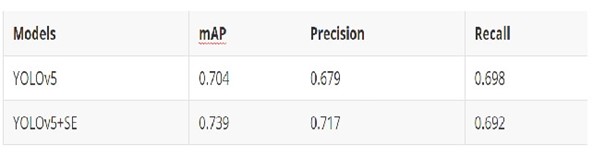
Changes Introduced by Adding Attention Mechanism:

3.5 Object/Object Tracking

Our tracker is built on top of the Deep SORT algorithm.

Algorithm Workflow:

1. The detector obtains bounding boxes (bbox).
2. Generate detections.
3. Kalman filter prediction.
4. Use the Hungarian algorithm to match the predicted tracks with the detections in the current frame (cascade matching and IOU matching).
5. Kalman filter update.

Due to time constraints, we did not implement this algorithm from scratch but chose to reference open-source code. You can find the code at this address: https://github.com/nwojke/deep_sort

3.6 Field Localization – Resnet18 Model

Paper: [1] Jiang W , Higuera J , Angles B , et al. Optimizing Through Learned Errors for Accurate Sports Field Registration[J]. 2019.

This method provides a way to project the coordinates of a point on the camera image to the actual coordinates on the field.

Model: By reproducing the paper, you can obtain a Resnet18 model to generate the projection matrix. You only need to project the center coordinates of the detected objects in the image using this model to get the global position of the object on the field.

3.7 Parameter Tuning Process

YOLOv5’s parameters can be configured in the specified YAML file or passed as additional parameters during runtime. Here are several types of parameters:

1. Network Configuration File:
   • Model depth and width.
   • Anchor settings with three predefined modes.
   • Backbone.
   • Head.
2. Initialization Hyperparameters:
   • Hyperparameters (hpy), including learning rate (lr), weight decay, momentum, and image processing parameters.
   • Training hyperparameters, including configuration file selection, training image size, pretraining, batch size, number of epochs, etc.

Due to time and resource constraints, we mainly focused on tuning three parameters:

• conf-thres: Confidence threshold (default = 0.25).
• NMS: Non-Maximum Suppression (default = false).
• epochs: Number of training epochs (default = 300).

3.7.1 Confidence

Confidence = 0.25, NMS = default (0%), epochs = default (300)

Confidence tuning is mostly done through empirical adjustments based on results, somewhat resembling the process of tuning a PID controller.

A lower confidence value means that objects that do not closely match target features may be selected.

3.7.2 Non-Maximum Suppression (NMS)

Confidence = default (0.25), NMS = 0%, epochs = default (300):

• NMS = 0%
• NMS = 20%
• NMS = 40%
• NMS = 60%
• NMS = 80%
• NMS = 100%

During tuning, we found that changing the NMS value did not significantly affect the detections. This might be because the Anchor parameters were already set for small object detection.

We also observed that NMS had a greater impact on detections when confidence was decreased, which is logically consistent.

Confidence = 0.15, NMS = variable, epochs = default (300):

• NMS = 0%
• NMS = 20%
• NMS = 40%
• NMS = 60%
• NMS = 80%
• NMS = 100%

3.7.3 Number of Training Epochs

Confidence = 0.15, NMS = 20%, epochs = variable (0-300)

3.7.4 Unexpected Issues

Loss Became NaN in the Logs

Solution: Parameter tuning based on the MindSpore documentation.

4. Results Evaluation

The results evaluation process was largely reflected during the parameter tuning phase.

5. Conclusion

In this assignment, our group used two main models, YOLOv5s and ResNet18. We optimized our models by introducing the Attention Mechanism (SE), although due to time constraints, C++ optimization and acceleration were not fully implemented. Overall, our model achieved a high level of completion.

We used MindSpore as the framework for this assignment, but we encountered some issues:

1. The official MindSpore documentation seemed to lack version management, leading to incorrect results when following the provided instructions step by step.

2. Compatibility issues with different versions of MindSpore’s CANN and CUDA were not properly documented, causing us to take many detours.

3. MindSpore performed poorly on Windows systems, lacking GPU support and generating various strange errors. Therefore, we eventually deployed it on a server.

4. The error-solving suggestions in the Ascend ModelZoo were not very helpful, and most of the errors were resolved based on our own experience.

5. MindSpore, being a relatively niche framework, often lacked suitable solutions to problems online, and its resources were not as rich as those of frameworks like PyTorch.

6. In summary, MindSpore shows promise for the future, but it still has some room for improvement.

6、References

[1] Jiang W , Higuera J , Angles B , et al. Optimizing Through Learned Errors for Accurate Sports Field Registration[J]. 2019.

[2] Jie Hu, Li Shen, Gang Sun; Proceedings of the IEEE Conference on Computer Vision and Pattern Recognition (CVPR), 2018, pp. 7132-7141